Spread Windows Forms Product Documentation

Highlighting Rules

You can use this rule to highlight data that meets one of the following conditions:

is greater than a value
is less than a value
is between a high and low value
is equal to a value
contains a specific value
is a date that occurs in a particular range
is either unique or duplicated elsewhere in the worksheet

After you choose one of the options above, enter a value or formula against which each cell is compared. If the cell data satisfies that criteria, then the formatting is applied.

You can select a predefined highlight style or create a custom highlight style. The following rules are highlight style rules:

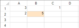
This figure illustrates the following example.

An Example of Highlighting Rule

Using Code

Set the properties of the rule class.
Apply the formatting.

Example

This example code creates the between values rule and uses the SetConditionalFormatting method to apply the rule.

private void Form1_Load(object sender, EventArgs e)
        {
            fpSpread1.Sheets[0].Cells[0, 0].Value = 3;
            fpSpread1.Sheets[0].Cells[1, 0].Value = 2;
            fpSpread1.Sheets[0].Cells[1, 1].Value = 5;
            fpSpread1.Sheets[0].Cells[0, 2].Value = 1;
        }

        private void button1_Click(object sender, EventArgs e)
        {
          FarPoint.Win.Spread.BetweenValuesConditionalFormattingRule between = new FarPoint.Win.Spread.BetweenValuesConditionalFormattingRule(true, 10, false, 20, false);
        between.FirstValue = 10;
        between.SecondValue = 20;
        between.IsNotBetween = true;
        between.BackColor = Color.Bisque;
        fpSpread1.ActiveSheet.SetConditionalFormatting(1, 1, between);
        }

Private Sub Form1_Load(ByVal sender As System.Object, ByVal e As System.EventArgs) Handles MyBase.Load
        fpSpread1.Sheets(0).Cells(0, 0).Value = 3
        fpSpread1.Sheets(0).Cells(1, 0).Value = 2
        fpSpread1.Sheets(0).Cells(1, 1).Value = 5
        fpSpread1.Sheets(0).Cells(0, 2).Value = 1
    End Sub

    Private Sub Button1_Click(ByVal sender As System.Object, ByVal e As System.EventArgs) Handles Button1.Click
        Dim between As New FarPoint.Win.Spread.BetweenValuesConditionalFormattingRule(True, 10, False, 20, False)
        between.FirstValue = 10
        between.SecondValue = 20
        between.IsNotBetween = True
        between.BackColor = Color.Bisque
        fpSpread1.ActiveSheet.SetConditionalFormatting(1, 1, between)
    End Sub

Using the Spread Designer

In the work area, select the cell or cells for which you want to set the conditional format.
Under the Home menu, select the Conditional Formatting icon in the Style section, then select the Highlight Cells Rules option, and then choose the condition.
From the File menu choose Apply and Exit to apply your changes to the component and exit Spread Designer.

Highlighting Rules

Using Code

Example

Using the Spread Designer

See Also